ShallowWaters.jl - A type-flexible 16-bit shallow water model
![]()
![]()

A shallow water model with a focus on type-flexibility and 16-bit number formats. ShallowWaters allows for Float64/32/16, Posit32/16/8, BFloat16, LogFixPoint16, Sonum16, Float32/16 & BFloat16 with stochastic rounding and in general every number format with arithmetics and conversions implemented. ShallowWaters also allows for mixed-precision and reduced precision communication.
ShallowWaters uses an energy and enstrophy conserving advection scheme and a Smagorinsky-like biharmonic diffusion operator. Tracer advection is implemented with a semi-Lagrangian advection scheme. Strong stability-preserving Runge-Kutta schemes of various orders and stages are used with a semi-implicit treatment of the continuity equation. Boundary conditions are either periodic (only in x direction) or non-periodic super-slip, free-slip, partial-slip, or no-slip. Output via NetCDF.
Please feel free to raise an issue if you discover bugs or have an idea how to improve ShallowWaters.
Requires: Julia 1.2 or higher
How to use
RunModel initialises the model, preallocates memory and starts the time integration. You find the options and default parameters in src/DefaultParameters.jl (or by typing ?Parameter).
help?> Parameter
search: Parameter

  Creates a Parameter struct with following options and default values

  T::DataType=Float32                 # number format

  Tprog::DataType=T                   # number format for prognostic variables
  Tcomm::DataType=Tprog               # number format for ghost-point copies

  # DOMAIN RESOLUTION AND RATIO
  nx::Int=100                         # number of grid cells in x-direction
  Lx::Real=2000e3                     # length of the domain in x-direction [m]
  L_ratio::Real=2                     # Domain aspect ratio of Lx/Ly
  ...
They can be changed with keyword arguments. The number format T is defined as the first (but optional) argument of RunModel(T,...)
julia> Prog = run_model(Float32,Ndays=10,g=10,H=500,Fx0=0.12);
Starting ShallowWaters on Sun, 20 Oct 2019 19:58:25 without output.
100% Integration done in 4.65s.
or by creating a Parameter struct
julia> P = Parameter(bc="nonperiodic",wind_forcing_x="double_gyre",L_ratio=1,nx=128);
julia> Prog = run_model(P);
The number formats can be different (aka mixed-precision) for different parts of the model. Tprog is the number type for the prognostic variables, Tcomm is used for communication of boundary values.
Double-gyre example
You can for example run a double gyre simulation like this
julia> using ShallowWaters
julia> P = run_model(Ndays=100,nx=100,L_ratio=1,bc="nonperiodic",wind_forcing_x="double_gyre",topography="seamount");
Starting ShallowWaters on Sat, 15 Aug 2020 11:59:21 without output.
100% Integration done in 13.7s.
Sea surface height can be visualised via
julia> using PyPlot
julia> pcolormesh(P.η')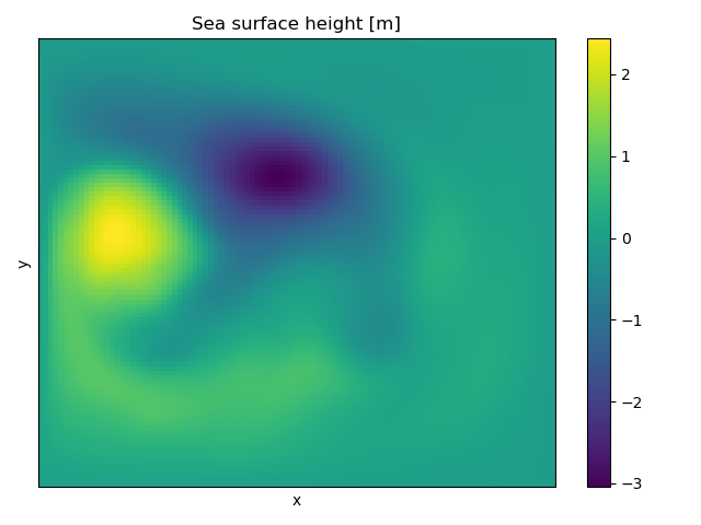
Or let's calculate the speed of the currents
julia> speed = sqrt.(Ix(P.u.^2)[:,2:end-1] + Iy(P.v.^2)[2:end-1,:])P.u and P.v are the u,v velocity components on the Arakawa C-grid. To add them, we need to interpolate them with Ix,Iy (which are exported by ShallowWaters.jl too), then chopping off the edges to get two arrays of the same size.
julia> pcolormesh(speed')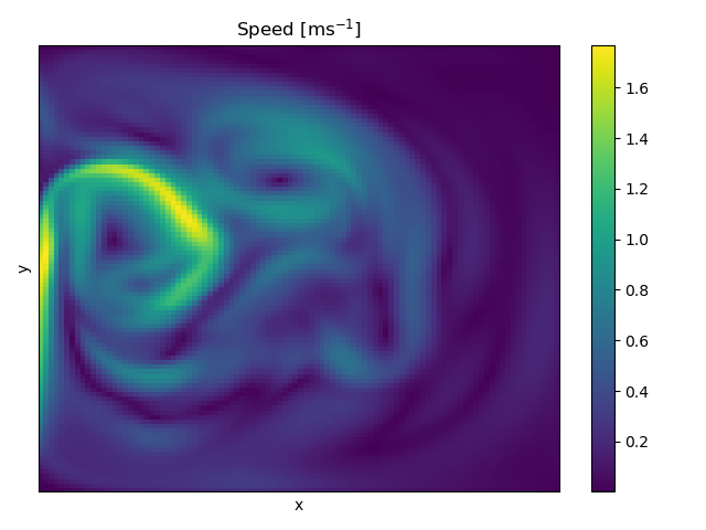
Such that the currents are strongest around the two eddies, as expected in this quasi-geostrophic setup.
(Some) Features
- Interpolation of initial conditions from low resolution / high resolution runs.
- Output of relative vorticity, potential vorticity and tendencies du,dv,deta
- (Pretty accurate) duration estimate
- Can be run in ensemble mode with ordered non-conflicting output files
- Runs at CFL=1 (RK4), and more with the strong stability-preserving Runge-Kutta methods
- Solving the tracer advection comes at basically no cost, thanks to semi-Lagrangian advection scheme
- Also outputs the gradient operators ∂/∂x,∂/∂y and interpolations Ix, Iy for easier post-processing.
Installation
ShallowWaters.jl is a registered package, so simply do
julia> ] add ShallowWatersReferences
ShallowWaters.jl was used and is described in more detail in
Klöwer M, Düben PD, Palmer TN. Number formats, error mitigation and scope for 16-bit arithmetics in weather and climate modelling analysed with a shallow water model. Journal of Advances in Modeling Earth Systems. doi: 10.1029/2020MS002246
Klöwer M, Düben PD, Palmer TN. Posits as an alternative to floats for weather and climate models. In: Proceedings of the Conference for Next Generation Arithmetic 2019. doi: 10.1145/3316279.3316281
The equations
The non-linear shallow water model plus tracer equation is
      ∂u/∂t + (u⃗⋅∇)u - f*v = -g*∂η/∂x - c_D*|u⃗|*u + ∇⋅ν*∇(∇²u) + Fx(x,y)     (1)
      ∂v/∂t + (u⃗⋅∇)v + f*u = -g*∂η/∂y - c_D*|u⃗|*v + ∇⋅ν*∇(∇²v) + Fy(x,y)     (2)
      ∂η/∂t = -∇⋅(u⃗h) + γ*(η_ref - η) + Fηt(t)*Fη(x,y)                       (3)
      ∂ϕ/∂t = -u⃗⋅∇ϕ                                                          (4)
with the prognostic variables velocity u⃗ = (u,v) and sea surface heigth η. The layer thickness is h = η + H(x,y). The Coriolis parameter is f = f₀ + βy with beta-plane approximation. The graviational acceleration is g. Bottom friction is either quadratic with drag coefficient cD or linear with inverse time scale r. Diffusion is realized with a biharmonic diffusion operator, with either a constant viscosity coefficient ν, or a Smagorinsky-like coefficient that scales as ν = cSmag*|D|, with deformation rate |D| = √((∂u/∂x - ∂v/∂y)² + (∂u/∂y + ∂v/∂x)²). Wind forcing Fx is constant in time, but may vary in space.
The linear shallow water model equivalent is
      ∂u/∂t - f*v = -g*∂η/∂x - r*u + ∇⋅ν*∇(∇²u) + Fx(x,y)     (1)
      ∂v/∂t + f*u = -g*∂η/∂y - r*v + ∇⋅ν*∇(∇²v) + Fy(x,y)     (2)
      ∂η/∂t = -H*∇⋅u⃗ + γ*(η_ref - η) + Fηt(t)*Fη(x,y)         (3)
      ∂ϕ/∂t = -u⃗⋅∇ϕ                                           (4)
ShallowWaters.jl discretises the equation on an equi-distant Arakawa C-grid, with 2nd order finite-difference operators. Boundary conditions are implemented via a ghost-point copy and each variable has a halo of variable size to account for different stencil sizes of various operators.